Deep Learning Assignment

1. Evaluate the Variants of the Basic Convolution Function

The basic convolution function is a fundamental operation in signal processing and deep learning, defined as:

$(f * g) (t) = \int_{- \infty}^{\infty} f (τ) g (t - τ) d τ$

or its discrete equivalent. While this standard form is powerful, several variants have been developed to address specific computational needs, data characteristics, or hardware constraints. Evaluating these variants highlights trade-offs between computational efficiency, memory usage, and representational capacity.

Key Variants and Evaluation

1. Transposed Convolution (or Deconvolution/Fractionally-Strided Convolution):
- Purpose: Essential for upsampling, such as in decoder stages of autoencoders or Generative Adversarial Networks (GANs), to increase spatial resolution.
- Evaluation: It’s not the mathematical inverse of convolution but rather performs a convolution with a specific structure that achieves upsampling. It can suffer from the “checkerboard artifact” due to uneven overlaps, though this can be mitigated.
2. Dilated Convolution (or Atrous Convolution):
- Purpose: Increases the receptive field of the filter without increasing the number of parameters or sacrificing spatial resolution (stride = 1).
- Evaluation: By inserting zeros between kernel elements (dilation rate), it captures wider context. This is highly effective in tasks like semantic segmentation (e.g., in DeepLab) where capturing multi-scale context is crucial, offering a good balance between context and computational cost.
3. Separable Convolution:
- Purpose: Dramatically reduces computational cost and the number of parameters.
- Evaluation: There are two main types:
  - Spatial Separable: Breaks a 2D convolution into two 1D convolutions (e.g., a $3 \times 3$ kernel becomes $3 \times 1$ followed by $1 \times 3$ ). This significantly reduces operations but is less common in deep learning.
  - Depthwise Separable (most common): Splits the convolution into two steps:
    1. Depthwise Convolution: A single filter is applied to each input channel independently.
    2. Pointwise Convolution: A $1 \times 1$ convolution is used to combine the outputs across channels.
  - This variant (used heavily in architectures like MobileNets) is far more efficient than standard convolution but might compromise a minor degree of representational power.

2. analyzing the Bidirectional RNNs in The Long Short-Term Memory and Other Gated RNNs

The Bidirectional Recurrent Neural Network (BiRNN) is an architectural enhancement that significantly boosts the performance of sequential models like the Long Short-Term Memory (LSTM) and Gated Recurrent Unit (GRU) by allowing them to utilize information from both the past and the future of a sequence.

Architecture and Function

A standard (or unidirectional) RNN/LSTM processes a sequence strictly from $t = 1$ to $t = T$ , basing its current state only on past information. A BiRNN addresses this limitation by running two independent RNN layers over the input sequence:

Forward Layer: Processes the input sequence from left-to-right (from $t = 1$ to $T$ ), capturing past context ( $h_{t}$ ).
Backward Layer: Processes the input sequence from right-to-left (from $t = T$ to $1$ ), capturing future context ( $h_{t}$ ).

The final output or hidden state $h_{t}$ at any time step $t$ is the concatenation or a summation of the hidden states from both layers: $h_{t} = [h_{t}; h_{t}]$ .

200

Analysis and Significance

When applied to LSTMs or GRUs (creating BiLSTMs or BiGRUs), the BiRNN structure leverages the gating mechanisms of these cells—the input, forget, and output gates—to control the flow of information in both directions. This is crucial for tasks where the context is symmetric, meaning a word’s meaning is influenced by words before it and words after it.

Advantages:

Richer Context: BiLSTMs/BiGRUs possess a complete understanding of the sequence by having access to all surrounding data points.
Superior Performance: They consistently yield state-of-the-art results in tasks like Named Entity Recognition (NER), Machine Translation, and speech recognition, where future context is vital for disambiguation.

Disadvantage: They require all input data to be present before prediction can begin, making them unsuitable for real-time or streaming applications where latency is critical.

3. the Encoder-Decoder Sequence-to-Sequence Architectures

The Encoder-Decoder architecture is the foundational framework for Sequence-to-Sequence (Seq2Seq) tasks, designed to map an input sequence to an output sequence where the lengths may differ (e.g., machine translation). This model revolutionized tasks in Natural Language Processing (NLP), such as text summarization and machine translation, before the rise of the pure Transformer.

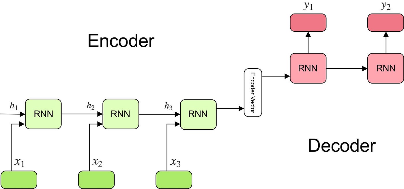
Components and Function

Encoder:
- Typically an RNN (LSTM or GRU), the encoder processes the entire input sequence $X = (x_{1}, \dots, x_{N})$ one token at a time.
- It compresses all the information into a single, fixed-length vector known as the context vector (C). This vector is the final hidden state of the encoder and aims to encapsulate the semantic summary of the input.
Decoder:
- Also typically an RNN, the decoder is initialized with the encoder’s context vector (C) as its initial hidden state.
- It generates the output sequence $Y = (y_{1}, \dots, y_{M})$ one token at a time, autoregressively. Each output $y_{t}$ is predicted based on the context vector $C$ and the previously generated outputs $(y_{1}, \dots, y_{t - 1})$ .

Limitations and Advancements

The primary limitation of the basic architecture is forcing the entire input sequence into a fixed-size context vector, leading to an information bottleneck. For long input sequences, the model often forgets the initial parts of the sequence.

This was largely solved by the Attention Mechanism, which allows the decoder to selectively “attend” (focus) on the most relevant parts of the input sequence at each step of the output generation, vastly improving performance on longer sequences. Modern models like the Transformer are also based on the encoder-decoder structure but replace the recurrent layers entirely with attention mechanisms.

Encoder And Decoder- Neural Machine Learning Language Translation Tutorial With Keras- Deep Learning

4. remembering the Optimization for Long-Term Dependencies, Explicit Memory

The challenge of long-term dependencies in Recurrent Neural Networks (RNNs) stems from the vanishing and exploding gradient problem during Backpropagation Through Time (BPTT). This makes it difficult for a standard RNN to pass information effectively across many time steps. Optimization efforts have largely focused on two strategies: architectural changes and Explicit Memory mechanisms.

Architectural Optimization (Gated RNNs)

The primary solution involves replacing the simple RNN unit with Gated Recurrent Units, most notably the Long Short-Term Memory (LSTM) and Gated Recurrent Unit (GRU). These are forms of implicit memory:

LSTM: Introduces a Cell State ( $C_{t}$ ), a linear “conveyor belt” designed to maintain information over long periods. Three gates (Forget, Input, Output) use element-wise multiplication ( $⊙$ ) and sigmoid functions to regulate the flow of information into and out of the cell state, preventing the gradient from decaying or exploding.
GRU: A simpler, two-gate variant (Update and Reset) that achieves similar performance with fewer parameters.

These gates create paths with derivatives near 1, effectively solving the vanishing gradient problem and allowing the model to optimize for long-term dependencies.

Explicit Memory Augmentation

Beyond gating, models can be augmented with Explicit Memory structures that function like external, addressable databases:

Memory Networks (MemNets): Use a key-value structure where the model’s query (hidden state) interacts with a large external memory to retrieve relevant information.
Neural Turing Machines (NTMs): Combine a standard neural network (controller) with a memory bank. The controller learns to perform read and write operations on the memory via soft, differentiable attention mechanisms, providing the model with a form of working memory that can store and retrieve data over arbitrary time steps.

5. applying the Challenge of Long-Term Dependencies, Echo State Networks

The Echo State Network (ESN) is a type of Recurrent Neural Network (RNN) designed specifically to circumvent the difficulty of training long-term dependencies in conventional RNNs caused by the vanishing/exploding gradient problem. ESNs achieve this through a unique, highly simplified training approach known as Reservoir Computing.

Evasion of the Gradient Challenge

Standard RNNs use Backpropagation Through Time (BPTT) to train all weights, including the recurrent weights responsible for carrying long-term memory, which is where the gradient issues arise. ESNs eliminate this problem by:

Fixed Reservoir: The large, internal recurrent layer (the “reservoir”) has its connections and weights initialized randomly and they are never trained.
Echo State Property: The weights are scaled to satisfy the Echo State Property, which ensures the network’s current state is a fading function of its entire input history. This non-linear reservoir thus transforms the input sequence into a high-dimensional temporal signal, effectively creating a rich, dynamic memory.

Application of Long-Term Memory

Since the reservoir weights are fixed, the network’s temporal dynamics are established before training. The only component trained is a simple linear output layer ( $W^{o u t}$ ) connecting the reservoir states to the desired output.

Training becomes a simple, efficient linear regression task on the collected reservoir states. This linear training step sidesteps the complex non-linear optimization inherent in BPTT, making ESNs incredibly fast to train and highly effective for tasks like time-series prediction and modeling of dynamical systems where capturing long-range temporal patterns is essential.

6. create these Large-Scale Deep Learning, Computer Vision, Speech Recognition models

The creation of Large-Scale Deep Learning models for specialized fields like Computer Vision and Speech Recognition relies on three critical pillars: Architecture, Data, and Training at Scale. These models have millions or billions of parameters and require massive computational resources.

Computer Vision Models (LVMs)

Architecture: The foundation is the Convolutional Neural Network (CNN) (e.g., ResNet, VGG), which excels at extracting spatial hierarchies of features from image pixels. Modern large-scale vision models (LVMs) increasingly adopt the Vision Transformer (ViT) architecture, which processes images as sequences of patches and uses self-attention to capture global relationships more effectively.
Data: Training requires massive, high-quality, labeled datasets (e.g., ImageNet, COCO). Techniques like data augmentation (rotating, cropping, flipping images) are crucial to enhance data diversity and prevent overfitting.
Scale: Training on datasets containing millions or billions of images requires distributed training across multiple GPUs or TPUs.

Speech Recognition Models (ASR)

Architecture: Modern Automatic Speech Recognition (ASR) models use End-to-End (E2E) architectures, typically a Transformer-based Encoder-Decoder model (like OpenAI’s Whisper) or a Conformer, which integrates the strengths of CNNs and Transformers. The encoder processes the audio features (e.g., Mel spectrograms), and the decoder generates the output text.
Data: Success demands massive, diverse audio datasets (hundreds of thousands of hours) paired with accurate text transcripts. Weak supervision (using noisy web-scale data) and self-supervised learning (like wav2vec 2.0) are essential to learn robust representations from unlabeled audio before fine-tuning.
Scale: E2E models consolidate the entire traditional speech pipeline (acoustic, lexicon, and language models), requiring immense parallel computation during training to optimize the entire sequence-to-sequence transformation at once.

Harsh RB

Explorer