NIC Assignment

1. Explain hill climbing algorithm.

Hill Climbing is a heuristic search algorithm used in Artificial Intelligence for solving optimization problems. It is based on the idea of iterative improvement, where the algorithm continuously moves towards a better solution by evaluating neighboring states and choosing the one with the highest value (or lowest cost, depending on the problem). The process resembles climbing a hill where the aim is to reach the top or a peak.

The algorithm starts with an initial solution and evaluates it using a heuristic function (also called the evaluation function). From the current state, it examines the neighboring states (possible solutions derived by making small changes). If a neighbor has a better evaluation score than the current state, the algorithm moves to that state. This process is repeated until no better neighbor exists, at which point the algorithm stops.

Hill Climbing is simple and efficient, but it has certain limitations. It can get stuck in situations such as:

Local Maxima – A point where the algorithm cannot find a better neighbor, even though higher peaks exist elsewhere.
Plateaus – A flat region where neighboring states have the same value, making it hard to decide the direction.
Ridges – Areas where the global maximum can only be reached by moving away from the steepest ascent temporarily.

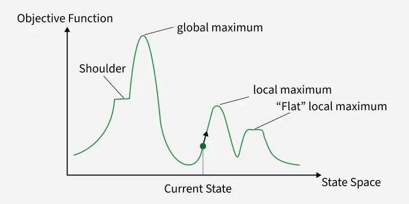
To overcome these issues, variations of hill climbing are used, such as Steepest-Ascent Hill Climbing (choosing the best among all neighbors), Stochastic Hill Climbing (choosing randomly among better neighbors), and Random-Restart Hill Climbing (restarting the process with different initial states to avoid being stuck).

2. Explain Ant colony optimization algorithm.

Ant Colony Optimization (ACO) is a probabilistic optimization algorithm inspired by the foraging behavior of real ants. In nature, ants search for food and communicate with each other using chemical substances called pheromones. When an ant finds food, it returns to the colony while laying down pheromones on the path. Other ants sense these pheromone trails and are more likely to follow them. Over time, shorter and better paths accumulate stronger pheromone concentrations, guiding most ants toward the optimal route.

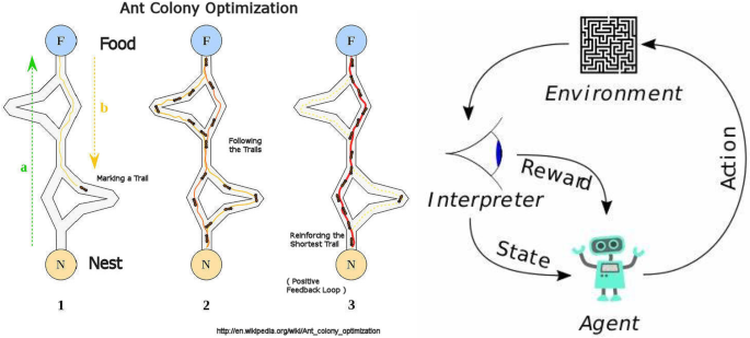
ACO uses this natural mechanism to solve combinatorial optimization problems, such as the Traveling Salesman Problem (TSP), routing, scheduling, and network optimization.

The algorithm works as follows:

Initialization – Place multiple artificial ants randomly on possible solutions.
Solution Construction – Each ant builds a solution by moving step by step through available choices. The probability of choosing the next step depends on two factors:
- Pheromone level (τ): Indicates how desirable the path is based on past ant experiences.
- Heuristic value (η): Represents problem-specific information, such as the inverse of distance in TSP.
Pheromone Update – After all ants complete their paths, pheromone trails are updated.
- Good solutions receive stronger pheromone deposits.
- Some pheromones evaporate over time to avoid convergence to suboptimal solutions.
Iteration – Steps are repeated until convergence or stopping criteria are met.

ACO has several strengths:

It is adaptive and works well in dynamic environments.
It naturally balances exploration (searching new paths) and exploitation (using the best-known paths).

However, it also has limitations:

It may converge prematurely to a non-optimal solution.
Computational cost increases with problem complexity.

3. Explain basic integrated & fire neuron model.

The Integrate-and-Fire (I&F) neuron model is one of the simplest and most widely used mathematical models to describe the functioning of biological neurons. It captures the essential mechanism of how neurons process and transmit information through electrical impulses, known as spikes or action potentials.

In this model, the neuron is represented as an electrical circuit that integrates incoming signals over time. When other neurons send input signals, they are modeled as currents entering the neuron. The neuron’s membrane potential (voltage across the cell membrane) increases as it integrates these inputs. This is mathematically described using a differential equation that accumulates the effect of incoming currents.

Once the membrane potential reaches a certain threshold value, the neuron is said to “fire” an action potential. At this moment, the model emits a spike, which is the way neurons communicate with each other. Immediately after firing, the membrane potential is reset to a baseline level (called the resting potential) and may enter a refractory period, during which it cannot fire again. This reset mechanism ensures discrete and time-separated spikes.

The basic integrate-and-fire model ignores many biological complexities but is powerful for understanding information processing in large neural networks. Variants of the model include the leaky integrate-and-fire (LIF) model, where the membrane potential naturally decays over time if no inputs are received. This leakage makes the model more biologically realistic, as real neurons lose charge due to ion leakage across membranes.

The I&F model is widely used in computational neuroscience, artificial neural networks, and neuromorphic computing because of its simplicity and efficiency. While it does not capture detailed ion channel dynamics (as in the Hodgkin-Huxley model), it provides a balance between biological plausibility and computational efficiency, making it suitable for simulating large-scale networks of spiking neurons.

4. Discuss the recurrent network.

A Recurrent Neural Network (RNN) is a type of artificial neural network where connections between units form a directed cycle, allowing information to persist over time. Unlike feedforward networks, where data flows only in one direction (from input to output), recurrent networks have feedback loops that enable them to maintain a kind of internal memory. This makes RNNs particularly powerful for handling sequential or time-dependent data.

Structure:

An RNN consists of input, hidden, and output layers. The hidden layer plays a key role because its neurons not only receive the current input but also feedback from their own previous state. This recurrence allows the network to “remember” past information and use it to influence the current output. Mathematically, the hidden state at time step t depends on both the input at t and the hidden state at t–1.

Applications:

Recurrent networks are widely used in:

Natural Language Processing (NLP): language modeling, text prediction, and machine translation.
Speech Recognition: processing audio signals over time.
Time Series Prediction: forecasting stock prices, weather, or traffic flow.
Control Systems and Robotics: where sequential decision-making is required.

Advantages:

Ability to capture temporal dependencies in sequential data.
Can model complex relationships where current outputs depend on previous inputs.

Limitations:

Vanishing and exploding gradient problems during training, making it hard to learn long-term dependencies.
Computationally expensive for very long sequences.
Struggles with long-range memory unless improved variants are used.

Variants:

To overcome limitations, advanced recurrent architectures were developed:

Long Short-Term Memory (LSTM): introduces memory cells and gates to retain information over longer periods.
Gated Recurrent Unit (GRU): a simplified version of LSTM with fewer parameters.

5. Genetic algorithm with example.

A Genetic Algorithm (GA) is a search and optimization technique inspired by the principles of natural selection and genetics in biological evolution. It is widely used in Natural Inspired Computing to solve complex optimization problems where traditional methods are inefficient.

Working Principle:

Genetic algorithms work with a population of candidate solutions, called chromosomes, which evolve toward better solutions over successive generations. Each chromosome is typically represented as a string (binary, real-valued, or symbolic). The process involves the following steps:

Initialization: Generate an initial population randomly.
Evaluation: Measure the fitness of each chromosome using a fitness function, which defines how good a solution is for the given problem.
Selection: Choose parent chromosomes based on their fitness. Fitter individuals have a higher chance of being selected (survival of the fittest).
Crossover (Recombination): Combine parts of two parents to produce offspring, introducing new solutions.
Mutation: Randomly alter some parts of chromosomes to maintain diversity and avoid premature convergence.
Replacement: Form a new population by replacing weaker solutions with newly generated ones.
Termination: Repeat until a stopping condition is met (e.g., maximum generations or satisfactory solution).

Example: Traveling Salesman Problem (TSP)

In the TSP, the goal is to find the shortest possible route visiting all cities exactly once and returning to the starting point.

Chromosome Representation: A chromosome can represent a sequence of cities (e.g., [A, B, C, D, E]).
Fitness Function: The inverse of the total distance traveled (shorter routes have higher fitness).
Crossover: Two parents exchange segments of their city sequences to create valid new routes.
Mutation: Swap two cities in the sequence to explore new possibilities.
Process: Over generations, the algorithm evolves routes that are progressively shorter, converging toward an optimal or near-optimal solution.

6. Explain simulated Annealing Algorithm.

Simulated Annealing (SA) is a probabilistic optimization algorithm inspired by the annealing process in metallurgy, where a material is heated to a high temperature and then cooled slowly to remove defects and reach a more stable crystalline structure. In Natural Inspired Computing, SA is used as a global optimization method to avoid being trapped in local optima, making it suitable for large and complex search problems.

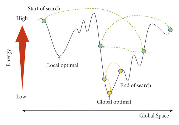
Working Principle: The algorithm starts with an initial solution and an initial “temperature” parameter. At each step, a new candidate solution (neighbor) is generated by making a small random change to the current solution. The decision to move to this new solution depends on two cases:

If the new solution is better (lower cost or higher fitness), it is always accepted.
If the new solution is worse, it may still be accepted with a probability that decreases as the system cools. This probability is defined by:

P = e^{- Δ E / T}

where:

$Δ E$ = difference in cost (worse – current),
$T$ = current temperature.

As the algorithm progresses, the temperature is gradually reduced following a cooling schedule (e.g., exponential decay or linear decrease). This mechanism ensures exploration at higher temperatures and exploitation at lower temperatures.

Advantages:

Avoids local minima by occasionally accepting worse solutions.
Simple and flexible, applicable to many optimization problems.

Limitations:

Convergence is slow if the cooling schedule is too gradual.
Sensitive to parameter choices (initial temperature, cooling rate).

Example: Consider the Traveling Salesman Problem (TSP): a salesman must visit all cities exactly once and return to the start. SA begins with a random tour and iteratively swaps cities to generate new tours. At high temperature, even longer tours may be accepted, allowing exploration. As temperature decreases, the algorithm favors shorter tours, gradually converging to a near-optimal path.

7. Explain network architecture.

Network architecture refers to the design and structure of artificial neural networks (ANNs), which are computational models inspired by the human brain. ANNs are built from interconnected processing units called neurons, organized in layers that work collectively to learn and solve complex problems.

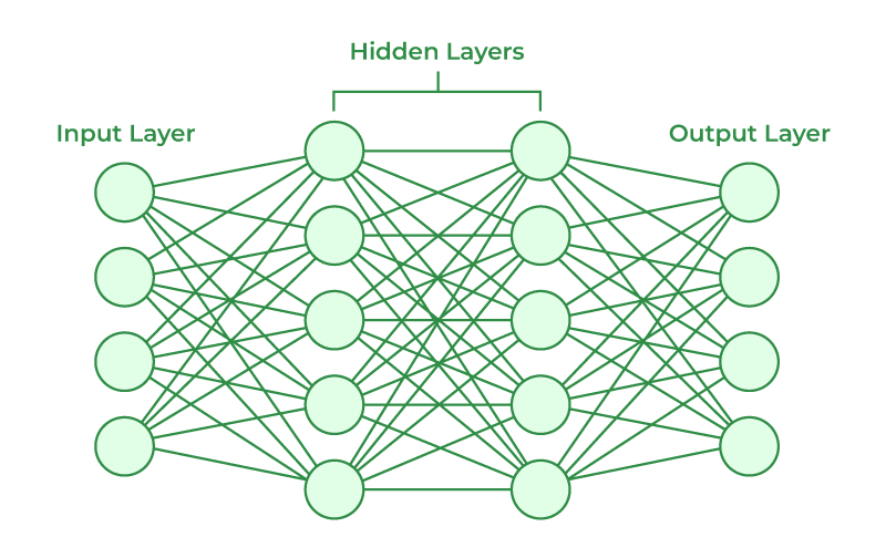
Basic Components:

Input Layer: Receives raw data from the environment (e.g., images, text, signals). Each node represents a feature.
Hidden Layers: Perform computations by transforming inputs through weighted connections and activation functions. Multiple hidden layers allow networks to capture nonlinear patterns.
Output Layer: Produces the final result, such as a class label, probability, or numeric prediction.

Connections:

Each connection between neurons has a weight, which determines the influence of one neuron on another.
A bias term is added to improve flexibility.
An activation function (e.g., sigmoid, ReLU, tanh) introduces nonlinearity, enabling the network to model complex functions.

Types of Architectures:

Feedforward Neural Networks (FNN): Data flows strictly from input to output, without cycles. Useful for static pattern recognition.
Recurrent Neural Networks (RNN): Include feedback loops, making them suitable for sequential data (speech, text, time series).
Convolutional Neural Networks (CNN): Specialized for image and spatial data, inspired by the visual cortex.
Deep Neural Networks (DNN): Multiple hidden layers that learn hierarchical feature representations.

Training Process:

Training involves adjusting weights using optimization algorithms (like Gradient Descent).
The backpropagation algorithm computes gradients to minimize error between predicted and actual outputs.

Applications in NIC:

Pattern Recognition: Face, speech, and handwriting recognition.
Optimization: Solving scheduling, routing, and control problems.
Natural Language Processing: Machine translation, sentiment analysis.
Bio-inspired Systems: Modeling brain processes and adaptive decision-making.

8. Explain mccullah and pits model.

The McCulloch and Pitts (MCP) model, proposed in 1943 by Warren McCulloch (a neuroscientist) and Walter Pitts (a logician), is considered the first mathematical model of a neuron. It laid the foundation for Artificial Neural Networks (ANNs), forming a bridge between neuroscience and computation. This model is simple yet powerful, showing how networks of simple processing units (neurons) could perform logical and computational tasks.

Structure of MCP Neuron:

The MCP model represents a neuron as a binary threshold unit:

Inputs ( $x_{1}, x_{2}, \dots, x_{n}$ ) – These are signals received by the neuron from the external environment or other neurons.
Weights ( $w_{1}, w_{2}, \dots, w_{n}$ ) – Each input is associated with a weight that represents the importance of that input.
Summation Function – Computes the weighted sum of all inputs:

S = i = 1 \sum n w_{i} x_{i}

Threshold (θ) – A fixed value that determines neuron activation.
Activation Function (Step Function) – If the weighted sum $S \geq θ$ , the neuron “fires” (output = 1), otherwise it does not (output = 0).

Mathematical Representation:

y = {10 if \sum w_{i} x_{i} \geq θ if \sum w_{i} x_{i} < θ

Working: The MCP neuron essentially acts as a binary classifier. It decides whether to activate or not based on the weighted sum of inputs compared to the threshold. This makes it function like a simple logic gate.

Example: To implement an AND gate:

Inputs: $x_{1}, x_{2} \in {0, 1}$
Weights: $w_{1} = 1, w_{2} = 1$
Threshold: $θ = 2$
Output: Fires (1) only if both inputs are 1, otherwise 0.

Similarly, OR and NOT gates can also be modeled.